Pictures of lines

Thus far I have introduced the uncertainty principle and used it to demonstrate that quantum mechanics behaves quite oddly, to say the least, from the point of view of classical logic. What makes the uncertainty principle highly interesting for quantum theory is its almost complete independence of any physical details; it is indeed an inherent property of mathematics used to describe the quantum world, and is thus necessarily present in all physical systems. This, in fact, suggests that the uncertainty principle is a derivative property of something more fundamental and perhaps more elementary. Here we will leave the uncertainty principle behind and explore this idea by considering the geometry of the quantum state space; it turns out that a useful approach to shed some light on the logic of quantum mechanics is to draw lines.

Quantum states are represented by vectors in a vector space, or more precisely, by linear subspaces of the state space¹. For the sake of visualisation, we will concentrate on a two-dimensional Euclidean space, which is a fancy name for the familiar coordinate plane. So in our case each state corresponds to a line in the plane passing through the origin (it could also be the case that the state is the origin or the entire plane). Here is an example of two states, let’s call them red and blue:

We should immediately ask, what are the suitable logical operations for ‘and’ and ‘or’? Since the lines represent the physical states, we want to be able to say something like ‘The system is in the blue and red state’ as well as ‘The system is in the blue or red state’². We will start with ‘and’ as it is perhaps more intuitive.

For the states represented by lines, ‘and’ is defined simply as the intersection of the lines³. Recall that ‘and’ is represented by the symbol . That is, to say that the system is in ‘blue and red’ state is to find where on our plane the state is simultaneously blue and red. Clearly, there are two possibilities here; firstly, if the lines happen to coincide (i.e. they were in fact the same line) the ‘and’ operation is redundant and the intersection is just the original line; in general, however, the lines will be different and will intersect only at the origin. In our example case this looks like:

One could think that the definition of ‘or’ is as simple as that of ‘and’; it is tempting to define ‘or’ as the union of the two lines, the system is either in the blue state or in the red one. This naive definition is, however, implausible both mathematically and physically. Mathematically, the union of two lines is no longer a linear subspace of the plane; indeed, we agreed that each state is either a line, the origin or the entire plane, but the union of two lines is some kind of skewed cross. Thus this definition of ‘or’ does not preserve the structure we started with. Physically, the definition has even more catastrophic consequences; it implies that measuring the state should yield either ‘blue result’ or ‘red result’, depending on which state we happen to measure. We know, however, that this is not the case, instead the measurement will result in some linear combination (i.e. some mixture of both coordinates) of ‘blue’ and ‘red’, this is the so called ‘principle of superposition’. This principle, in fact, already suggests the appropriate definition of ‘or’.

‘Or’ in our linear representation is defined as ‘the smallest linear subspace of the plane containing both lines’. Recall that or is represented by the symbol . Again, two things could happen, the first one being the redundant case when the two lines coincide and nothing happens, and for two distinct lines their ‘or’ is the entire plane. This definition overcomes both problems mentioned above; it guarantees that the resulting state is a linear subspace and it accounts for superposition. Thus for the lines we started with, the ‘or’ operation looks like:

Equipped with these logical operations, let us reconsider the distributive law once again. For that, let’s add a third line, called green, to our plane:

Recall that the classical distributive law asserts:

⁴

Now, using the definitions of ‘and’ and ‘or’ as above, let us figure out visually how both sides of this equality look like. These will turn out to be quite different.

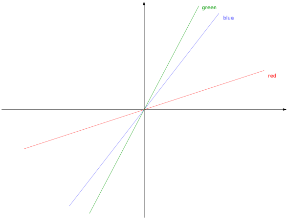
We start from the left-hand side: green and (blue or red). We already know what (blue or red) is from one of the pictures above, it is simply the entire plane. Thus we need the intersection of the green line with the plane, which is just the green line itself:

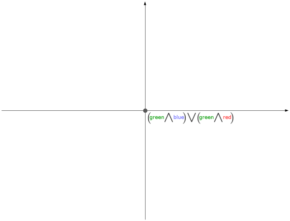
For the right-hand side, both terms in brackets are intersections of two distinct lines; (green and blue) and (green and red). Thus they are both equal to the origin, as before. Now the result is the smallest linear subspace containing the origin, hence just the origin itself:

We have therefore managed to show that the distributive law does not hold for these definitions of ‘and’ and ‘or’. What is fascinating about this example is its similarity to the one with ‘quantum cyclist’ discussed last time, which required a complicated construction and the uncertainty principle. This visual approach demonstrates that non-distributivity of quantum logic is really a consequence of geometry of vector spaces.

---

¹ mathematically state space is a Hilbert space

² or the probabilities of these in the case of quantum physics

³ more precisely, intersection of the linear subspaces of the Hilbert space

⁴ For the intuition behind this, see the beginning of the previous post or the very end of the first post